
Once you have collected multiple traces using ProfilingManager, exploring them
individually to find performance problems becomes impractical. Bulk trace
analysis lets you query a dataset of traces simultaneously to:
- Identify common performance regressions.
- Calculate statistical distributions (for example, P50, P90, P99 latency).
- Find patterns across several traces.
- Find outlier traces to understand and debug performance issues.
This section demonstrates how to use the Perfetto Python Batch Trace Processor to analyze startup metrics across a set of locally stored traces and locate outlier traces for deeper analysis.
Design the query
The first step to perform a bulk analysis is to create a PerfettoSQL query.
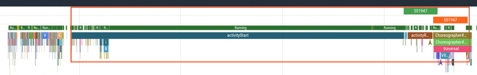
In this section, we present an example query that measures app startup latency.
Specifically, you can measure the duration from activityStart to the first
frame generated (the first occurrence of the Choreographer#doFrame slice) to
measure app startup latency that is within your app's control. Figure 1 shows
the section to query.
CREATE OR REPLACE PERFETTO FUNCTION find_slices(pattern STRING) RETURNS
TABLE (name STRING, ts LONG, dur LONG) AS
SELECT name,ts,dur FROM slice WHERE name GLOB $pattern;

CREATE OR REPLACE PERFETTO FUNCTION generate_start_to_end_slices(startSlicePattern STRING, endSlicePattern STRING, inclusive BOOL) RETURNS
TABLE(name STRING, ts LONG, dur LONG) AS
SELECT name, ts, MIN(startToEndDur) as dur
FROM
  (SELECT S.name as name, S.ts as ts, E.ts + IIF($inclusive, E.dur, 0) - S.ts as startToEndDur
  FROM find_slices($startSlicePattern) as S CROSS JOIN find_slices($endSlicePattern) as E
  WHERE startToEndDur > 0)
GROUP BY name, ts;

SELECT ts,name,dur from generate_start_to_end_slices('activityStart','*Choreographer#doFrame [0-9]*', true)
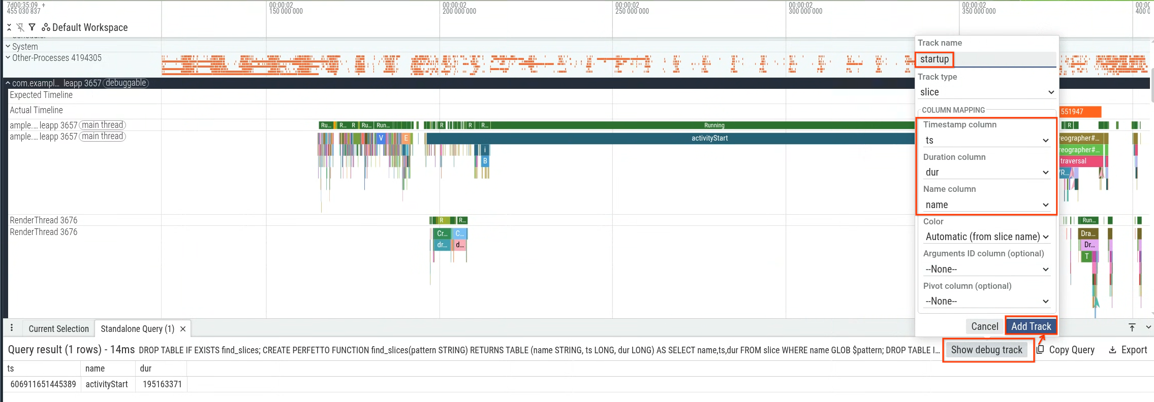
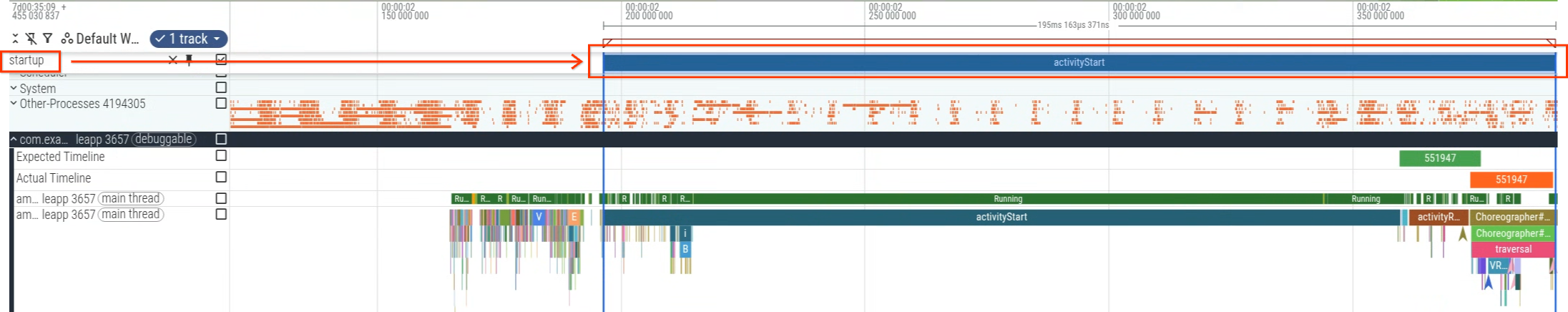
You can execute the query within the Perfetto UI and then use the query results to generate a debug track (Figure 2) and visualize it within the timeline (Figure 3).
Set up the Python environment
Install Python on your local machine and its required libraries:
pip install perfetto pandas plotly
Create the bulk trace analysis script
The following sample script executes the query in multiple traces using
Perfetto's Python BatchTraceProcessor.
from perfetto.batch_trace_processor import BatchTraceProcessor
import glob
import plotly.express as px

# Collect all trace files in the local directory
traces = glob.glob('*.perfetto-trace')

if not traces:
    print("No .perfetto-trace files found in the current directory.")
    exit(1)

if __name__ == '__main__':
    # Process all traces in parallel to aggregate metrics across runs
    with BatchTraceProcessor(traces) as btp:
        query = """
        CREATE OR REPLACE PERFETTO FUNCTION find_slices(pattern STRING) RETURNS
        TABLE (name STRING, ts LONG, dur LONG) AS
        SELECT name,ts,dur FROM slice WHERE name GLOB $pattern;

        CREATE OR REPLACE PERFETTO FUNCTION generate_start_to_end_slices(startSlicePattern STRING, endSlicePattern STRING, inclusive BOOL) RETURNS
        TABLE(name STRING, ts LONG, dur LONG) AS
        SELECT name, ts, MIN(startToEndDur) as dur
        FROM
          (SELECT S.name as name, S.ts as ts, E.ts + IIF($inclusive, E.dur, 0) - S.ts as startToEndDur
          FROM find_slices($startSlicePattern) as S CROSS JOIN find_slices($endSlicePattern) as E
          WHERE startToEndDur > 0)
        GROUP BY name, ts;

        SELECT ts,name,dur / 1000000 as dur_ms from generate_start_to_end_slices('activityStart','*Choreographer#doFrame [0-9]*', true)
        """
        df = btp.query_and_flatten(query)
        # Plot the distribution of startup times, tracking trace file paths on
        # hover
        violin = px.violin(df, x='dur_ms', hover_data='_path', title='startup time', points='all')
        violin.show()
Understand the script
When you run the Python script, it performs the following actions:
- The script searches in your local directory for all Perfetto traces suffixed
with
.perfetto-traceand uses them as source traces for analysis. - It runs a bulk trace query that computes the subset of startup time
corresponding to the time from the
activityStarttrace slice to the first frame generated by your app. - It plots the latency in milliseconds using a violin plot to visualize the distribution of startup times.
Interpret the results
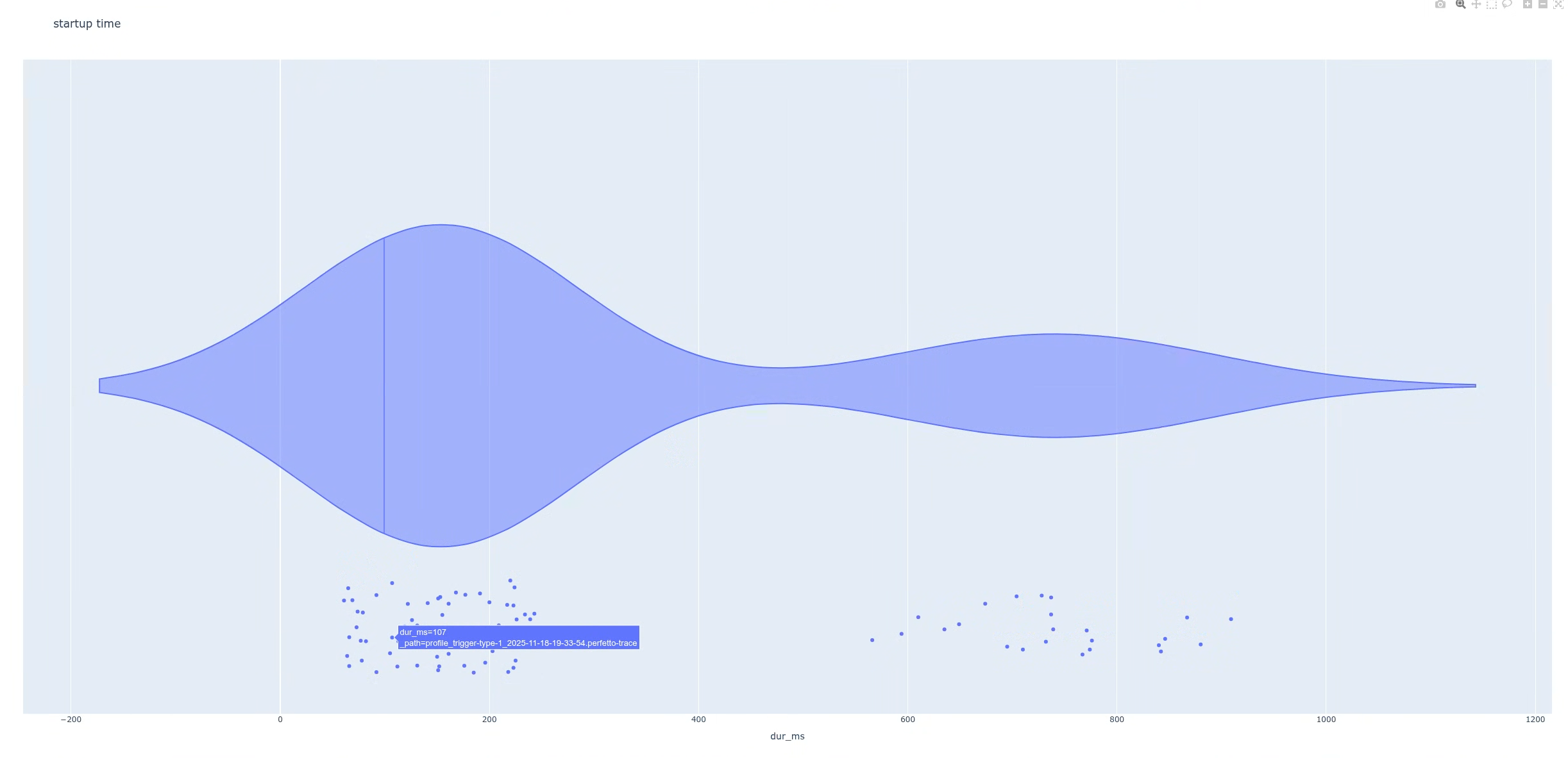
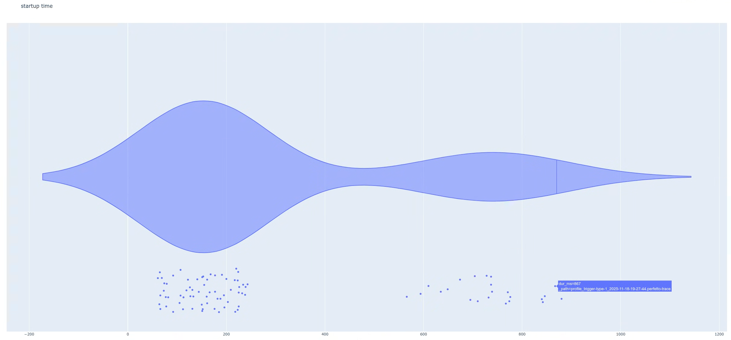
After you execute the script, the script generates a plot. In this case, the plot shows a bimodal distribution with two distinct peaks (Figure 4).
Next, find the difference between the two populations. This helps you examine individual traces in more detail. In this example, the plot is set up so that when you hover over the data points (latencies), you can identify the trace filenames. You can then open one of the traces that is part of the high-latency group.
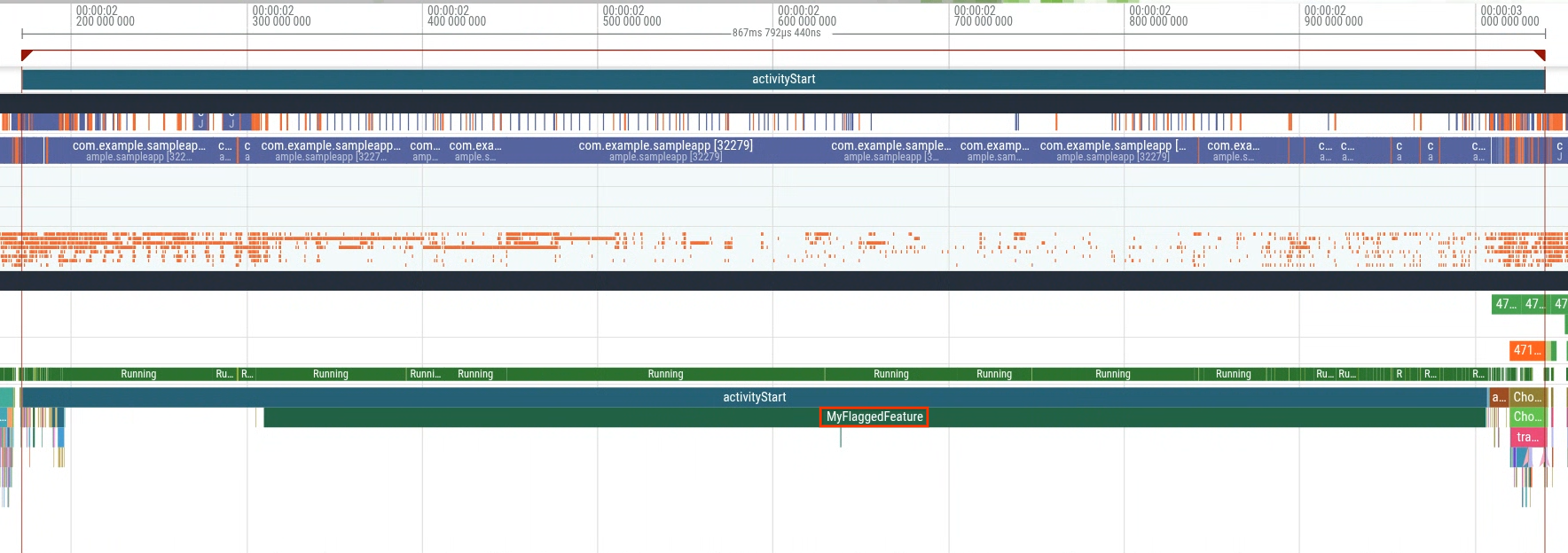
When you open a trace from the high-latency group (Figure 5), you will find an
extra slice named MyFlaggedFeature running during startup (Figure 6).
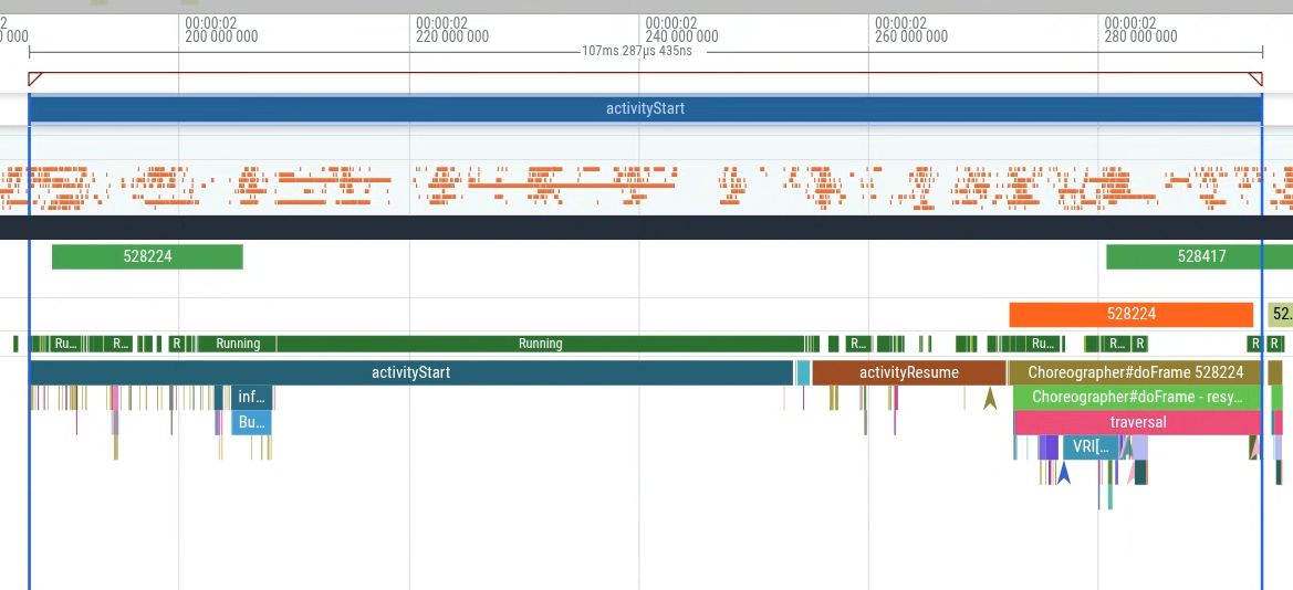
Conversely, selecting a trace from the lower-latency population (the leftmost
peak) confirms the absence of that same slice (Figure 7). This comparison
indicates that a specific feature flag, enabled for a subset of users, triggers
the regression.
This example demonstrates one of the many ways you can use bulk trace analysis. Other use cases include extracting statistics from the field to gauge impact, detecting regressions, and more.